Trice Command-Line Interface and Examples
Contents
- 1. Common information
- 2. Further examples
- 2.1. Automated pre-build insert command example
- 2.2. Some Log examples
- 2.3. Logging over a display server
- 2.4. Logfile output
- 2.5. Binary Logfile
- 2.6. TCP4 output
- 2.7. TCP4 input
- 2.8. UDP4 input
- 2.9. Stimulate target with a user command over UART
- 2.10. Explore and modify tags and their colors
- 2.11. Location Information
- 3. Visualization output with -vis
- 4. Setting up the LabPlot Demo
The trice tool is very easy to use even it has a plenty of options. Most of them normally not needed. The trice tool can be started in several modes (sub-commands), each with several mandatory or optional switches. Switches can have a single parameter string or not.
trice sub-command -switch1 -switch2 parameter -switch3 ...
Which sub-command switches are usable for each sub-command is shown with trice help -all. This gives also information about their default values.
Info for a special sub-command is shown with trice help -log for example.
- The command history is usable for example inside the bash, simply enter CTRL-R and start typing
trice...and you can select from the history. - The most convenient way is to use trice inside scripts like in this example.
1. Common information
trice h -allshows all options of the current version.trice verprints version information.trice sshows you all found serial ports for your convenience.trice l -p COM17could fail if something is wrong. Additional switches are for help tracking the issue:- Use log witch
-s[howInputBytes]to check if any bytes are received at all.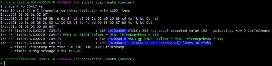
- With
-debugyou can see the [T]COBS packages and decoded Trice packages.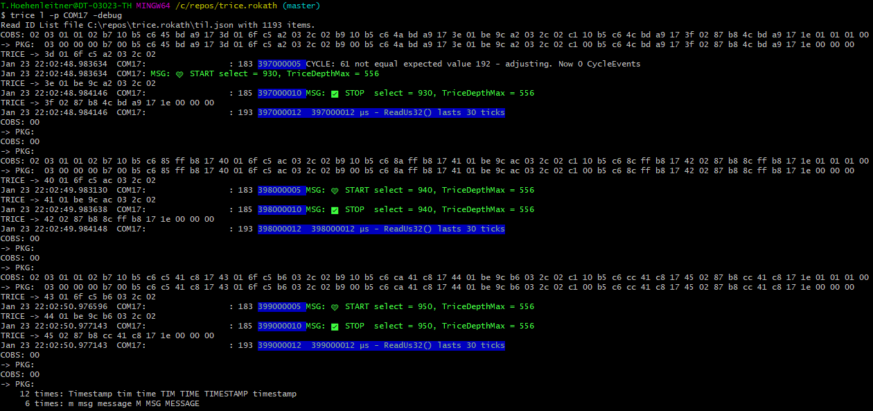
- Use log witch
-
trice iin the root of your project parses all source files for Trice macros, adds automatically ID´s if needed and updates a file named til.json containing all ID´s with their format string information. To start simply generate an empty file named til.json in your project root. You can addtrice ito your build process and need no further manual execution. trice dsstarts a display server listening on default ip address 127.0.0.1:61487 or any specified value. This is possible also on a remote device, lets say with ip address 192.168.1.200.trice l -p COM18 -dssends the log strings to a display server with default ip address 127.0.0.1:61487 or any specified value, if for example-ipa 192.168.1.200the trice logs go to the remote device. You can start several trice log instances, all transmitting to the same display server.
2. Further examples
2.1. Automated pre-build insert command example
- Scan directories
../src,../lib/srcand./to insert the IDs there and extend list file../../../til.json
trice i -v -i ../../../til.json -src ../src -src ../lib/src -src ./
This is a typical line you can add to your project as an automatic pre-compile step.
2.2. Some Log examples
- Log trice messages on COM3 8N1 115200 baud
trice log -i ./myProject/til.json -p=COM3
- Log trice messages on COM3 8N1 9600 baud and use default til.json
trice l -s COM3 -baud=9600
2.3. Logging over a display server
- Start displayserver on ip 127.0.0.1 (localhost) and port 61497
trice ds
- Log trice messages on COM3 and display on display server
trice l -ds -p COM3
- Shutdown remote display server on IP 192.168.1.23 port 45678
trice sd -r 192.168.1.23:45678
The IP address and port are free selectable. Using a display server, allows to watch the logs of one or many MCUs on a local or remote machine with the same or different display servers.
A local Trice instance sends Trice messages to a display server only, when a log line is complete (if consisting of several Trices). By using the CLI switches -prefix and -suffix you can decorate the loglines target specific to distinguish them in the output window(s).
2.4. Logfile output
trice l -p COM3 -logfile auto
This creates a new logfile 2022-05-16_2216-40_trice.log with the actual timestamp on each Trice start.
trice l -p COM3 -logfile trice.log
This creates a new logfile trice.log on first start and appends to it on each next Trice start.
Logfiles are text files one can see with 3rd party tools. Example: cat trice.log. They contain also the PC reception timestamps if where enabled.
2.5. Binary Logfile
trice l -p COM3 -binaryLogfile auto
This creates a new binary logfile 2022-05-16_2216-40_trice.bin with the actual timestamp on each Trice start.
trice l -p COM3 -binaryLogfile trice.bin
This creates a new binary logfile trice.bin on first start and appends to it on each next Trice start.
Binary logfiles store the Trice messages as they come out of the target in binary form. They are much smaller than normal logfiles, but the Trice tool with the matching til.json is needed for displaying them and the PC timestamps are the displaying time: trice l -p FILEBUFFER -args trice.bin.
Recording happens before decoding, -pick, -ban, -logLevel, and visualization. These host options therefore do not remove received bytes from the binary recording, even with -logLevel off. Partial or malformed input is also recorded; a recording write failure is returned as an error. Data already lost or suppressed on the target cannot be recovered from this file.
Replay can use a different selection, for example trice log -p FILEBUFFER -args trice.bin -pick err -pick wrn. Keep the matching dictionary and decoding settings (encoding, framing, and encryption) with the recording. An explicit binary filename is appended to across runs; use a new filename when separate captures are needed. Keep binary recording disabled during replay, or write to a different file, never the replay input itself.
Binary logfiles are handy in the field for long data recordings.
When using RTT, the data are exchanged over a file interface. These binary logfiles are stored in the project [./temp] folder and accessible for later view: trice l -p FILEBUFFER -args ./temp/logfileName.bin. Of course the host timestamps are the playing time then.
2.6. TCP4 output
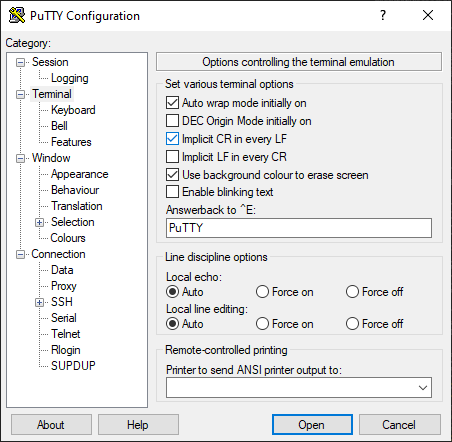
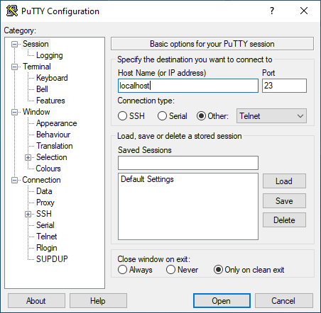
trice l -p COM3 -tcp 127.0.0.1:23
This additionally sends Trice output to a 3rd party TCP listener, for example like Putty:
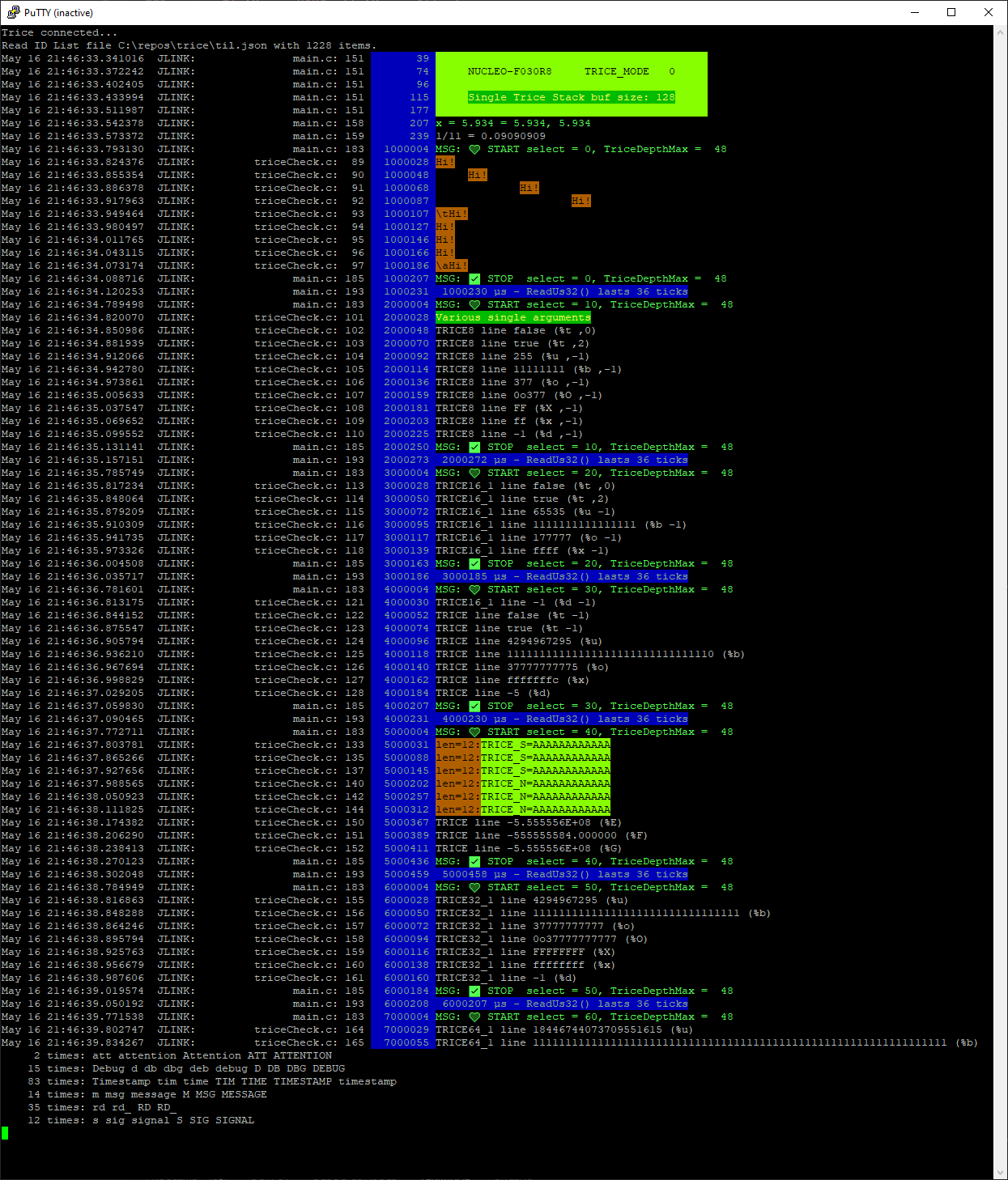
2.7. TCP4 input
trice l -p TCP4 -args "192.168.2.3:45678"
This expects a TCP4 server at IP address 192.168.2.3 with port number 45678 to read binary Trice data from.
2.8. UDP4 input
The pull request #529 introduces key enhancement:
    IPv4 UDP Receiver
    Adds support for receiving data over IPv4 using UDP. This enables integration with systems that broadcast or transmit telemetry, logs, or other messages over the network.
-port UDP4 Example
To receive Trice logs over IPv4 UDP, use the -port UDP4 option. By default, it listens on 0.0.0.0:17005, which accepts packets on all network interfaces. You can specify a different address or multicast group via -args.
trice log -p UDP4
2.9. Stimulate target with a user command over UART
Sometimes it is handy to stimulate the target during development. For that a 2nd screen is helpful what is possible using the display server option:
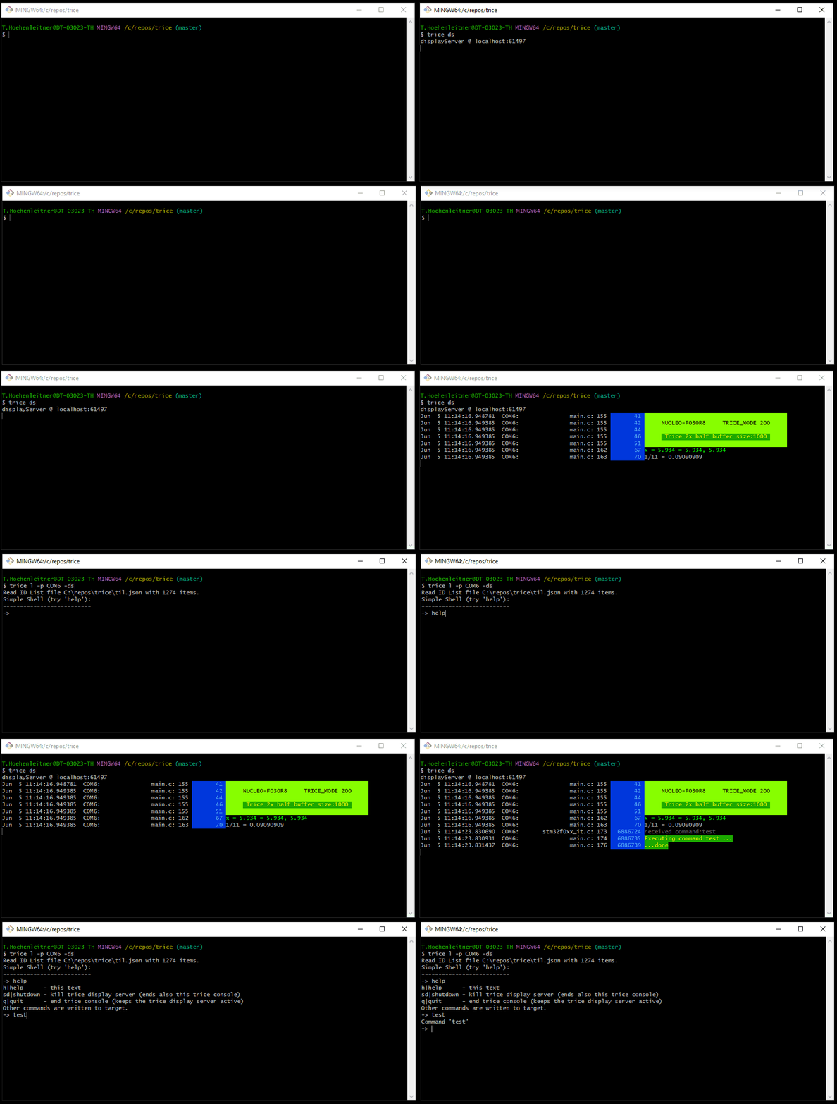
2.10. Explore and modify tags and their colors
See chapter Trice Tags and Color.
2.11. Location Information
The add, bind, insert, and clean commands generate the file selected by -li|locationInformation. Each entry stores one canonical source path and its line number:
{
  "1234": {
    "File": "examples/TriceABC/src/main.c",
    "Line": 42
  }
}
File is relative to -liRoot and always uses / separators. The default root is the directory containing the selected li.json. An explicit relative -liRoot is resolved from the current working directory. If a relative path cannot be represented, for example across Windows volumes, Trice stores a normalized absolute path without resolving symbolic links.
For example, when build/demoLI.json and examples/TriceABC/src/main.c are below the project directory, the default stores ../examples/TriceABC/src/main.c. To store a project-relative path instead, run:
trice insert -li build/demoLI.json -liRoot . -src examples/TriceABC
During logging, -liMaxDirs controls how much of the stored path is shown. Its default 0 shows only the filename. For examples/TriceABC/src/main.c, values 1, 2, and 3 show src/main.c, TriceABC/src/main.c, and the complete stored path respectively. Leading .. components describe the relation to -liRoot and are not displayed or counted. -liFmt continues to control the surrounding filename and line-number format.
Location information must match the exact firmware version. In field deployments, keeping li.json private and showing the numeric ID with -showID can be preferable. Use trice log -li off to disable location loading and display explicitly, even when a local LI exists.
LI also supplies source ownership evidence during ID processing. Keep the local file between Bind, Clean, and Insert runs even if you log without source locations: identical messages can occur at different sites, and TIL alone does not preserve their source associations. Removing LI can change ID reuse, particularly in partial scans. Passing -li off to an ID-processing command disables its LI use and generation too; use the switch only on log when you want to retain that evidence.
The repository’s active demo location tables are generated locally and ignored by Git; their build and ID-workflow scripts create a missing LI before processing IDs. A custom workflow must initialize a missing LI as well when LI is enabled, because ID processing requires an existing file. Preserve the matching LI as a firmware or capture artifact when later location lookup matters. Keeping LI in version control remains an option for applications that need to preserve source ownership across checkouts.
3. Visualization output with -vis
tlog and trice log support the same repeatable -vis option for sending selected numeric measurements to external visualization tools. Consumers can, for example, be LabPlot, Serial Studio, PlotJuggler, uPlot, Grafana, or a custom program; these names do not imply a tool-specific protocol. Trice itself does not draw a graph. It transforms one typed Trice message into one user-defined text record and writes that record to a file or UDP destination.
The syntax is:
-vis='<tag>:printf("<go-fmt>",<expression-list>)@<file-path-or-udp-sink>[;log=keep|drop]'
For example, this target message keeps its visualization details independent of the host tool:
TRice("imu:ax=%f,ay=%f,az=%f\n", aFloat(ax), aFloat(ay), aFloat(az));
It can be written as CSV:
tlog ... \
  -vis='imu:printf("%d,%0.3f,%0.3f,%0.3f\n",ts32,v0,v1,v2)@imu.csv'
or sent as one UDP datagram per record:
tlog ... \
  -vis='imu:printf("%0.3f,%0.3f,%0.3f\n",v0*0.5,v1*0.5,v2*0.5)@udp://127.0.0.1:7010;log=drop'
The selector matches the original Trice format prefix <tag>:. -pick and -ban run first. A message removed by either existing filter is therefore invisible both to normal output and to -vis.
The supported fields are:
id                unsigned Trice ID
ts                raw 16- or 32-bit Target-Stamp, with one width latched per rule
ts16              raw 16-bit Target-Stamp
ts32              raw 32-bit Target-Stamp
v0 ... v11        typed positional Trice values
The value fields are positional and can be reordered in the expression list. -vis does not extract names such as ax or rpm from the human-readable target format and does not accept those names as identifiers. For example, printf("%g,%g\n",v2,v0) deliberately emits the third value before the first. Structured Logging field names are not visualization expression identifiers; use v0 through v11 for this interface.
A Target-Stamp is an unscaled number. -vis does not assume that it represents time and does not perform unit conversion, wrap extension, or mixed-width reconstruction. Scaling is explicit in an expression, for example ts32*0.001. A rule may use ts16 or ts32, but not both. A generic ts rule is disabled with a warning if an otherwise eligible message later changes between 16 and 32 bits.
Separate rules make the expected stamp width explicit:
tlog ... \
  -vis='fast:printf("%d,%g\n",ts16,v0)@fast.csv' \
  -vis='slow:printf("%d,%g\n",ts32,v0)@slow.csv'
Expressions support decimal, floating-point, and hexadecimal literals, parentheses, unary minus, and +, -, *, /. A direct field retains its signed, unsigned, floating-point, or Boolean type. Arithmetic is evaluated as float64. A floating result used with an integer verb must be finite and inside the int64 range; it is then truncated toward zero.
The printf encoder supports:
integer:       %d %b %o %x %X
floating:      %f %e %E %g %G
generic:       %v
Boolean:       %t with a direct Boolean field
literal:       %%
formatting:    literal width and precision, such as %08x or %0.3f
%u, dynamic * width or precision, explicit argument indexes, string conversions, and other Go formatting verbs are not supported. The expression count must equal the number of consuming verbs. The encoder adds no implicit newline; include \n in the format when the receiving tool expects one. A one-line JSON record is possible as well:
tlog ... \
  -vis='imu:printf("{\"stamp\":%d,\"x\":%g,\"y\":%g,\"z\":%g}\n",ts32,v0,v1,v2)@udp://127.0.0.1:7011'
A bare path and file:<path> both select an append-only file:
@out.csv
@logs/imu.csv
@file:out.csv
Missing files are created. Rules using the same normalized file path share one open file. file://out.csv is rejected because standard URI parsing treats out.csv as a host, not as a relative path. Full file-URI semantics are not part of this implementation.
UDP destinations use:
@udp://127.0.0.1:7010
@udp://localhost:7010
The address is resolved and opened before decoding starts. File and UDP writes are synchronous. There is no queue, retry, reconnect, acknowledgement, TCP, WebSocket, or named-pipe support in this first implementation.
log=keep is the default and leaves the decoded message in normal output. log=drop removes it from normal output only after that rule has encoded and written the visualization record successfully. All overlapping rules are still attempted; one successful log=drop rule wins. An ignored record or a failed encoder or sink write does not drop the normal log.
Only fixed-width numeric Trice messages are eligible. The first twelve values are addressable as v0 through v11; additional values do not prevent a rule from using that addressable prefix and remain available to normal logging. Trice string, buffer, function-display, character, typeX0, CHAR, and DUMP inputs are not supported. Named values, specialized JSON or binary encoders, TCP, WebSocket, named pipes, and process pipes are deferred behind the same selector/encoder/sink separation. One eligible Trice must also form one complete log line by itself. Partial, multi-line, and multi-Trice lines continue through normal logging but are ignored by -vis; verbose mode reports every such occurrence.
At startup, each rule checks all matching historical til.json entries. Incompatible old entries are excluded independently, so one stale ID does not block another compatible ID. A rule with no compatible entry is disabled with a prominent warning. Rules are also disabled, never silently, after a generic Target-Stamp width conflict, an unsafe runtime expression conversion, or a sink failure. Normal logging continues.
4. Setting up the LabPlot Demo
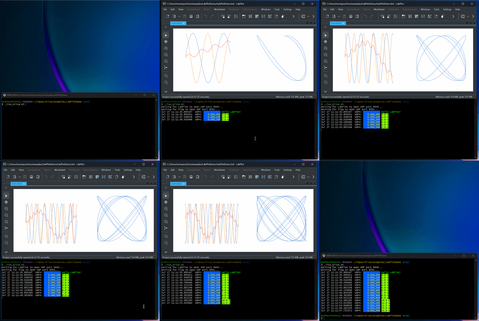
Select the preview to open the full animation.
This section uses LabPlot, a cross-platform interactive
plotting application. The finished, ready-to-run example is in
./examples/LabPlotDemo/; the guided learning path is in
./examples/LabPlotUser/. The project uses a UDP socket so that it can
display an endless stream without repeatedly importing files.
4.1. The common live-data format
Both producers describe the same three signals: x, y, and z. LabPlot
receives normalized numeric CSV records with this column layout:
time_s,x,y,z
The finished project predeclares the four numeric columns and performs one initial read while loading. This prepares LabPlot’s UDP socket before the first live record arrives. The UDP stream therefore needs no header row.
The LabPlot demo rate is 50 samples per second. The project retains 500 rows.
The time plot is configured for the last 500 values, so its horizontal
resolution stays constant and it always displays approximately the most
recent ten seconds. The Lissajous plot uses only the last 150 values, which
creates a moving three-second trace instead of an increasingly dense full
history. A slow phase modulation of y makes the figure change continuously.
The CSV producer sends this format directly. The Trice producer sends binary
Trice records to tlog; tlog decodes them and sends the same CSV format
onward. This separation means that one LabPlot project works for both
examples.
4.2. ./examples/DemoData_CSV
The CSV producer is a small C11 program
for Windows, macOS, and Linux. Each newline-terminated record contains
time_s,x,y,z, all represented as double; time is in seconds. It writes to
standard output by default, to a fresh file with --output FILE, or to UDP
with one record per datagram. Use --help for all options.
Both data producers require a C compiler and CMake 3.16 or newer. Run their
build.sh in Git Bash on Windows or a POSIX shell on macOS/Linux; restore its
executable permission with chmod +x build.sh if necessary. Executables are
installed in each project’s bin/, with intermediate files in build/.
For the CSV producer, the equivalent explicit CMake commands are:
cd examples/DemoData_CSV
cmake -S . -B build
cmake --build build --config Release
cmake --install build --config Release --prefix .
These commands also work in PowerShell. Its executable invocation is
.\bin\DemoData_CSV.exe; in Git Bash use ./bin/DemoData_CSV.
From the CSV project directory, try:
./build.sh
./bin/DemoData_CSV
./bin/DemoData_CSV --rate 50 --samples 500 --no-delay --header --output DemoData_CSV.csv
./bin/DemoData_CSV --udp 127.0.0.1 9000
Run these alternatives separately. The second command runs continuously at
50 Hz; interrupt it with Ctrl-C. The third writes ten seconds of data
without real-time waiting. On Windows PowerShell the UDP command is
.\bin\DemoData_CSV.exe --udp 127.0.0.1 9000.
For Serial Studio, choose Quick Plot (Comma Separated Values), then
Network Socket > UDP, set local port 9000, connect, and start the UDP
producer. Quick Plot treats all four columns as values. A custom project can
instead name the columns and use the first column as a timestamp axis. Its
input must be seconds,x,y,z; do not send --header on the live stream.
There is currently no versioned DemoData.ssproj in this repository.
Both producers use the following signal model for time t in seconds:
phase = (pi/3) * sin(2*pi*0.04*t)
x = sin(2*pi*0.70*t)
y = sin(2*pi*0.91*t + pi/2 + phase)
z = 0.6*sin(2*pi*0.13*t) + 0.2*x*y + pulse
The pulse has height 0.8 during the final 250 ms of every eight-second
interval. The slow phase modulation keeps the Lissajous plot moving. The
Trice producer calculates the signals as doubles and transmits float32 values.
After running build.sh inside ./examples/DemoData_CSV/, the executable is
installed in the local bin/ folder. You can run it there:
th@Thomass-MacBook-Pro-7 bin % ./DemoData_CSV --header -o log.csv
^C
th@Thomass-MacBook-Pro-7 bin % head log.csv
time_s,x,y,z
0.000000,0.000000,1.000000,0.000000
0.020000,0.087851,0.992854,0.027246
0.040000,0.175023,0.971519,0.053608
0.060000,0.260842,0.936300,0.078239
0.080000,0.344643,0.887701,0.100367
0.100000,0.425779,0.826415,0.119328
0.120000,0.503623,0.753319,0.134594
0.140000,0.577573,0.669459,0.145795
0.160000,0.647056,0.576032,0.152736
th@Thomass-MacBook-Pro-7 bin %
4.3. ./examples/DemoData_Trice
The Trice producer transports the
same signals as binary Trice records. Keep it inside the repository: its
CMake project uses the unchanged target library from ../../src.
Its build script prepares Bind and the
repository-root demoTIL.json before building; it requires the Trice host
tool in addition to the CSV producer’s prerequisites. Use this script rather
than plain CMake commands that omit Bind preparation. There is no private
til.json or fixed iD(1000) for this ID-free producer.
The 32-bit target stamp uses units of 10 ms: at 50 Hz the stamps are
0, 2, 4, .... Convert with seconds = ts/100.0 or
milliseconds = ts*10; ts*100 does not give seconds.
From examples/DemoData_Trice:
./build.sh
./bin/DemoData_Trice --samples 500 --no-delay
trice log -p FILEBUFFER -args DemoData_Trice.bin -pf TCOBS -til ../../demoTIL.json -li off
Without an output option, the producer recreates DemoData_Trice.bin in the
current directory (wb truncates its previous contents). --output FILE
selects another fresh file, --stdout writes binary data to standard output,
and --udp HOST PORT sends one complete TCOBS-framed record per datagram.
Without --samples it runs until interrupted. --samples 500 counts signal
samples, not all log records: startup and periodic diagnostic logs are extra.
Use --help for all options. On Windows PowerShell, run
.\bin\DemoData_Trice.exe with the same arguments.
After running build.sh inside ./examples/DemoData_Trice/, the executable is
installed in the local bin/ folder. You can run it there:
- Create binary log file:
th@Thomass-MacBook-Pro-7 bin % ./DemoData_Trice -o log.bin
Writing log.bin
^C
- Show logs in binary log file:
th@Thomass-MacBook-Pro-7 bin % tlog -p FILEBUFFER -args log.bin -til ../../../demoTIL.json -ulabel vis_demo | head
Jul 25 15:38:55.411676  FILEBUFFER:    0,000_000 0.000000,1.000000,0.000000
Jul 25 15:38:55.411691  FILEBUFFER:    0,000_002 0.087851,0.992854,0.027246
Jul 25 15:38:55.411705  FILEBUFFER:    0,000_004 0.175023,0.971519,0.053608
Jul 25 15:38:55.411714  FILEBUFFER:    0,000_006 0.260842,0.936300,0.078239
Jul 25 15:38:55.411725  FILEBUFFER:    0,000_008 0.344643,0.887701,0.100367
Jul 25 15:38:55.411737  FILEBUFFER:    0,000_010 0.425779,0.826415,0.119328
Jul 25 15:38:55.411752  FILEBUFFER:    0,000_012 0.503623,0.753319,0.134594
Jul 25 15:38:55.411765  FILEBUFFER:    0,000_014 0.577573,0.669459,0.145795
Jul 25 15:38:55.411776  FILEBUFFER:    0,000_016 0.647056,0.576032,0.152736
th@Thomass-MacBook-Pro-7 bin %
- Get CSV log file:
th@Thomass-MacBook-Pro-7 bin % tlog -p FILEBUFFER -args log.bin -til ../../../demoTIL.json -ulabel vis_demo -vis='vis_demo:printf("%0.3f,%0.3f,%0.3f,%0.3f\n",ts/100.0,v0,v1,v2)@log.csv;header="time_s,X,Y,Z\n";log=drop'
th@Thomass-MacBook-Pro-7 bin % head log.csv
time_s,X,Y,Z
0.000,0.000,1.000,0.000
0.020,0.088,0.993,0.027
0.040,0.175,0.972,0.054
0.060,0.261,0.936,0.078
0.080,0.345,0.888,0.100
0.100,0.426,0.826,0.119
0.120,0.504,0.753,0.135
0.140,0.578,0.669,0.146
0.160,0.647,0.576,0.153
th@Thomass-MacBook-Pro-7 bin %
The preceding file visualization rule recreates log.csv when tlog starts.
Its header is written once per sink; the quoted Go string supports \n.
Keep a single backslash in the shell’s single-quoted rule. log=drop suppresses
the successfully visualized records, while unrelated diagnostic logs remain.
For a live Serial Studio or other CSV viewer listening on UDP 9000, start
the decoder from the repository root before starting the binary producer:
trice log -p UDP4 -args 127.0.0.1:9001 -pf TCOBS -til demoTIL.json -ulabel vis_demo \
  -vis='vis_demo:printf("%0.6f,%0.6f,%0.6f,%0.6f\n",ts/100.0,v0,v1,v2)@udp://127.0.0.1:9000;log=drop'
In another terminal, also from the repository root:
examples/DemoData_Trice/bin/DemoData_Trice --udp 127.0.0.1 9001
On Windows the executable has an .exe suffix. The producer sends binary
Trice to 9001, not CSV; connecting it directly to the viewer on 9000
cannot work. The decoder converts its records to seconds,x,y,z. The LabPlot
launchers below automate this pipeline and its receiver-readiness checks.
4.4. Quick LabPlot demonstration
Install LabPlot 2.12 or newer. From the repository root, run one of these commands in a POSIX shell:
./examples/LabPlotDemo/run_csv.sh
./examples/LabPlotDemo/run_trice.sh
The script opens LabPlotDemo.lml and starts the selected producer. The first
script sends CSV directly to UDP port 9000. The second uses UDP port 9001
for binary Trice input and runs tlog as the decoder/forwarder to port 9000.
The script first waits until LabPlot has opened port 9000, then starts
tlog and waits until its input port 9001 is ready. Only then does it start
the Trice producer. The project opens one worksheet containing two plots side
by side:
Time series:x,y, andzversustime_s, always showing the last 500 values (ten seconds).Lissajous:yversusx, showing the last 150 values (three seconds) on fixed axes. The producer’s slow phase drift keeps the figure in motion.
Press Ctrl-C in the shell to stop the producer and decoder. If LabPlot is
not found automatically, set LABPLOT to its executable. On Windows, Git
Bash is a suitable shell; for example, use
LABPLOT=/c/Program\ Files/LabPlot/bin/labplot.exe.
4.5. Recreate the project in LabPlot
The following steps explain the project without requiring prior LabPlot
knowledge. Start run_csv.sh first and leave it running.
- Create a new LabPlot project and choose Add New > Live Data Source.
- Select Network UDP Socket, enter host
127.0.0.1and port9000. - Select the ASCII filter, comma as separator, and disable header detection.
Set all four data types to
Doubleand enter the namestime_s,x,y, andz. - Select Update on new data and retain
500values. This is the moving ten-second window at the demo’s 50 Hz rate. - Add a worksheet with a Cartesian plot. Add three XY curves. For every
curve choose
time_sas the X column and choosex,y, orzas the Y column. Enable the legend, label the axestime [s]andvalue, and enable automatic range scaling. In the plot’s range settings select Last values and enter500; otherwise the time axis keeps growing and the curves become increasingly compressed. - Add a second Cartesian plot to the same worksheet and select a horizontal
two-column worksheet layout. Add one XY curve with
xas its X column andyas its Y column. Select Last values and enter150. Fixed X and Y ranges from-1.1to1.1keep the scale stable while the three-second trace and the signal’s slow phase drift make the movement visible. - Save the project as
LabPlotUser.lml.
The finished LabPlotDemo.lml contains
these settings and no machine-specific paths. Open it manually if LabPlot is
already running. The LabPlotUser directory is the
place for your recreated LabPlotUser.lml; this section is its complete
rebuild guide. Both producers end at the same numeric UDP stream, for example
0.000000,0.000000,1.000000,0.000000.
Stop the producer and start the other launcher without changing the LabPlot
project. Keep only one producer sending to UDP 9000 and keep the live source
connected. The Trice launcher first waits for LabPlot on 9000, then for its
decoder on 9001. The supplied project predeclares all four numeric columns
and triggers an initial read when loaded so that LabPlot prepares its socket.
4.6. Troubleshooting and adaptations
labplotmust be discoverable or selected withLABPLOT. macOS also checks its standard application bundle. Windows searchesProgramFiles,ProgramW6432, andLOCALAPPDATAforlabplot.exeorlabplot2.exe; an explicitLABPLOToverride takes precedence.TLOGcan select a decoder outsidePATH. Producer executables stay in each demo’sbin/, with CMake intermediates inbuild/.- If the plots remain empty, verify that the producer is running and that no
other process owns UDP port
9000. - If
tlogreports that a-visrule was disabled because writing to port9000was refused, LabPlot was not listening when the decoder started. Restartrun_trice.sh; its readiness check normally prevents this race. Once a visualization rule is disabled, normal logging intentionally resumes, and itslog=dropoption is no longer applied. - For the Trice path, verify that
tlogis onPATHand thatdemoTIL.jsonis present at the repository root. SetTLOGorTRICE_TILwhen using non-default locations. - Keep the complete
-visexpression inside one pair of quotes. The semicolon separatesheaderandlogoptions inside that expression; it must not be interpreted by the shell. - To show another history length, change the retained-value count to
50 * seconds. For example,1000values show approximately 20 seconds. - The Trice path still uses UDP port
9001internally between the demo andtlog. If that port is busy, stop the other receiver or change it inrun_trice.shand its-argsvalue together.